핸즈온 머신러닝 4장 모델 훈련

핸즈온 머신리닝3 4장 모델훈련을 요약 정리해봅니다.

 

4장 모델 훈련 요약

주제	내용 요약
선형 회귀 (Linear Regression)	입력과 출력 사이의 선형 관계를 학습. 정규 방정식(normal equation)이나 SVD를 통해 해 구함.
경사 하강법 (Gradient Descent)	반복적으로 비용 함수 최소화. 학습률 설정이 중요하며, 세 가지 방법: 배치, 확률적, 미니배치.
다항 회귀 (Polynomial Regression)	비선형 관계를 모델링하기 위해 입력 특성의 다항식을 추가. 과적합과 과소적합에 주의 필요.
학습 곡선 (Learning Curve)	모델 성능을 시각화하여 과소적합/과적합 판단. 훈련/검증 오차 비교.
규제 (Regularization)	모델 복잡도를 줄여 과적합 방지. L1(라쏘)와 L2(릿지) 규제가 대표적.
조기 종료 (Early Stopping)	에포크 중 검증 오차가 증가하면 학습 중단. 과적합 방지 기법 중 하나.
로지스틱 회귀	회귀를 분류에 사용 결정경계 : 0과 1을 분류하는 경계( 직선, 평면, 초평면)

 

참조 코드 : https://github.com/rickiepark/handson-ml3

4.1 선형회귀

4.1.1 정규방정식(Normal Equation)

아래는 일반적인 선형회귀의 기울기와 절편을 구하는 공식입니다.

머신러닝에서 선형회귀를 구하는 최소제곱법(OLS)이라고 합니다.

$\hat{y}​=ax+b$
기울기 $a = \frac{\sum(x_i - \bar{x})(y_i - \bar{y})}{\sum(x_i - \bar{x})^2}$​
절편 $b = \bar{y} - a\bar{x}$

 

선형대수학을 통해 선형 회귀 모델의 최적 파라미터$\theta$를 직접계산할 수 있는데 이를 정규방정식이라고 합니다.

 

$\hat\theta=(X^TX)^{−1}X^Ty$

이 방식은 역행렬이 포함되어 $o(n^3)$의 계산량이 매우 큰 방식이라, 머신러닝에서는 잘 사용되지 않습니다.

 

$ y = 3*x + 4 $ 일 경우

import numpy as np
import statsmodels.api as sm

# 데이터 생성
np.random.seed(42)
m = 100
X = 2 * np.random.rand(m, 1)
y = 3 * X + 4 + np.random.randn(m, 1)

# 절편 추가
X_b = sm.add_constant(X)  # shape: (100, 2)

# 정규방정식 계산 (유사역행렬 사용)
theta_best = np.linalg.pinv(X_b.T @ X_b) @ X_b.T @ y

print("절편",theta_best[0])
print("기울기",theta_best[1])

 

절편 [4.21509616]
기울기 [2.77011339]

 

최소제곱법(OLS)으로 계산했을 때

직접 계산할 수도 있지만 statsmodels에 OLS를 사용할 수 있습니다.

 

직접 계산

a = np.sum((X - X.mean()) * (y - y.mean())) / np.sum((X - X.mean())**2)
b = y.mean() - a * X.mean()
print("절편",b)
print("기울기",a)

절편 4.215096157546746
기울기 2.770113386438484

 

OLS사용

model = sm.OLS(y, X_b)
results = model.fit()
print("절편",results.params[0])
print("기울기",results.params[1])

절편 4.215096157546749
기울기 2.7701133864384833

 

4.2 경사하강법

경사하강법은 **비용 함수(cost function)**를 최소화하기 위해 반복적으로 함수를 미분하여**기울기(gradient)**를 0으로 만드는 가중치(파라미터)를 조정하는 최적화 알고리즘입니다.

 

비용함수

평균제곱오차의 비용함수일 경우

 

$J(\theta)=\frac{1}{2m}\sum_{1}^{m} ( pred_i - y_i )^2$

 

미분했을 때 경사는 아래와 같이 계산됩니다.($\theta$의 편미분)

$∇​J(\theta)=\frac{1}{m}X^T(X_θ−y)$

 

error = y_pred - y_true          # shape: (m, 1)
gradient = (1/m) * X.T @ error   # shape: (n_features, 1)

 

기울기는 학습률( η) 만큼 반복적으로 반영됩니다.

θ:=θ−η⋅∇J(θ)

 

경사를 학습하는 단위에 따라 아래 3개로 달라집니다.

배치경사하강은 전체데이터셋을 사용하고, 확률적 경사하강(SGD)는 각 샘플 1개(1개 row)로 경사계산하며, 미니배치의 경우 배치크기(ex: 32개 16개)단위로 경사를 학습합니다.

배치 GD	전체 데이터셋 m개	$\theta := \theta - \eta \cdot \frac{1}{m} X^T(X\theta - y)$	느리지만 안정적
확률적 GD (SGD)	샘플 1개 $x^{(i)}$	$\theta := \theta - \eta \cdot \nabla J^{(i)}(\theta)$	빠르지만 진동 큼
미니배치 GD	배치 크기 b개	$\theta := \theta - \eta \cdot \frac{1}{b} X_b^T(X_b \theta - y_b)$	속도와 안정성 균형

 

import numpy as np
import statsmodels.api as sm

# 데이터 생성
np.random.seed(42)
m = 100
X = 2 * np.random.rand(m, 1)
y = 3 * X + 4 + np.random.randn(m, 1)
X_b = sm.add_constant(X)  # 절편항 추가

# 공통 설정
n_epochs = 50
learning_rate = 0.1

# 1. 배치 경사하강법
theta_batch = np.random.randn(2,1)
for epoch in range(n_epochs):
    gradients = 2/m * X_b.T @ (X_b @ theta_batch - y)
    theta_batch -= learning_rate * gradients

# 2. 확률적 경사하강법
theta_sgd = np.random.randn(2,1)
for epoch in range(n_epochs):
    for i in range(m):
        random_index = np.random.randint(m)
        xi = X_b[random_index:random_index+1]
        yi = y[random_index:random_index+1]
        gradients = 2 * xi.T @ (xi @ theta_sgd - yi)
        theta_sgd -= learning_rate * gradients

# 3. 미니배치 경사하강법
theta_mini = np.random.randn(2,1)
batch_size = 20
for epoch in range(n_epochs):
    indices = np.random.permutation(m)
    X_b_shuffled = X_b[indices]
    y_shuffled = y[indices]
    for i in range(0, m, batch_size):
        xi = X_b_shuffled[i:i+batch_size]
        yi = y_shuffled[i:i+batch_size]
        gradients = 2/batch_size * xi.T @ (xi @ theta_mini - yi)
        theta_mini -= learning_rate * gradients

print("배치 경사하강법 θ:", theta_batch.ravel())
print("확률적 경사하강법 θ:", theta_sgd.ravel())
print("미니배치 경사하강법 θ:", theta_mini.ravel())

배치 경사하강법 θ: [3.91125197 3.03839129]
확률적 경사하강법 θ: [4.00597696 2.27516959]
미니배치 경사하강법 θ: [4.21608467 2.77506002]

 

4.3 다항회귀

선형 모델을 확장하여 다항식으로 비선형관계를 학습하는 방법입니다.

 

$ y = \theta_0 + \theta_1x + \theta_2x^2 + \theta_3x^3 + \dots $

 

입력데이터 : 

$ y=0.5x^2 +1⋅x+2+ϵ $  
x : 평균 -3 표준편차 6인 정규분포

import numpy as np
import matplotlib.pyplot as plt
from sklearn.preprocessing import PolynomialFeatures
from sklearn.linear_model import LinearRegression
from sklearn.pipeline import Pipeline
import koreanize_matplotlib 

# 데이터 생성
np.random.seed(42)
m = 100 
X = 6 * np.random.rand(m, 1) - 3 
y = 0.5 * X**2 + X + 2 + np.random.randn(m, 1)

# 다항 회귀 모델
poly_reg = Pipeline([
    ("poly_features", PolynomialFeatures(degree=2, include_bias=False)),
    ("lin_reg", LinearRegression())
])
poly_reg.fit(X, y)

poly_reg_degree20 = Pipeline([
    ("poly_features", PolynomialFeatures(degree=20, include_bias=False)),
    ("lin_reg", LinearRegression())
])
poly_reg_degree20.fit(X, y)

# 예측용 입력값
X_new = np.linspace(X.min() - 1, X.max() + 1, 200).reshape(-1, 1)
y_pred = poly_reg.predict(X_new)
y_pred20 = poly_reg_degree20.predict(X_new)

# 시각화
plt.figure(figsize=(8, 5))
plt.scatter(X, y, label="데이터 분포", alpha=0.6)
plt.plot(X_new, y_pred, "r-", label="예측 (degree2)", linewidth=2)
plt.plot(X_new, y_pred20, "b-", label="예측 (degree20)", linewidth=2)
plt.xlabel("x")
plt.ylabel("y")
plt.ylim(y.min()-1,y.max()+1)
plt.title("다항 회귀 결과")
plt.legend()
plt.grid(True)
plt.tight_layout()
plt.show()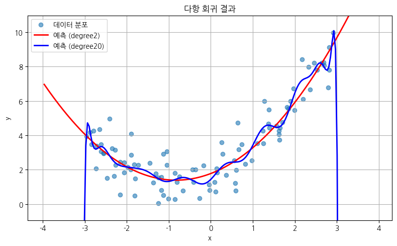

 

4.4 학습곡선 

모델이 과소적합(underfitting)또는 과적합(overfitting)되는지를 판단하는 중요한 진단 도구입니다.

학습곡선은 훈련세트 크기를 늘려가면서, 훈련오차와 검증오차의 편화를 시각화한 그래프입니다.

과적합인지, 과소작합인지를 그리고 데이터 양이 풍분한지 판단합니다.

learning_curve는 모델이 훈련데이터의 크기에 따라 어떻게 학습되는지를 분석하는데 사용됩니다.

from sklearn.model_selection import learning_curve

train_sizes, train_scores, val_scores = learning_curve(
    estimator, X, y, 
    train_sizes=np.linspace(0.1, 1.0, 5),
    cv=5,
    scoring="neg_mean_squared_error"
)

 

매개변수	설명
estimator	사용할 모델 (예: LinearRegression())
X, y	입력 특성과 타깃
train_size	훈련 데이터 크기의 비율/개수 (e.g., 10%~100%)
cv	교차검증 folds 수
scoring	평가 방식 (예: "neg_mean_squared_error", "accuracy")
shuffle	True일 경우 데이터를 섞음

 

반환값	설명
train_sizes	사용된 훈련 세트 크기 배열
train_scores	각 훈련 크기에서의 훈련 에러 (CV 평균)
val_scores	각 훈련 크기에서의 검증 에러 (CV 평균)

 

학습 곡선 해석 방법

1. 과소적합 : 훈련오차, 검증오차가 둘다 높은 상태에서 수렴

   모델이 너무 단순해서, 훈련이 안됨, 모델 복잡도 증가

2. 과적합 : 훈련오차, 검증오차가 모두 낮음 : 둘사이의 차이가 큼

   모델이 훈련데이터는 잘 맞추지만 검증데이터에서 성능이 낮음 

   규제 추가, 단순화, 학습데이터 증가

3. 적절한 모델

   훈련, 검증 오차 둘다 낮음 

import numpy as np
import matplotlib.pyplot as plt
from sklearn.model_selection import learning_curve
from sklearn.linear_model import LinearRegression
from sklearn.preprocessing import PolynomialFeatures
from sklearn.pipeline import Pipeline

# 1. 데이터 생성
np.random.seed(42)
m = 100
X = 6 * np.random.rand(m, 1) - 3
y = 0.5 * X**2 + X + 2 + np.random.randn(m, 1)

# 2. 다양한 차수의 다항 회귀 모델 준비
degrees = [1, 2, 20]
models = {}
for degree in degrees:
    model = Pipeline([
        ("poly_features", PolynomialFeatures(degree=degree, include_bias=False)),
        ("lin_reg", LinearRegression())
    ])
    models[degree] = model

# 3. 학습 곡선 계산
results = {}
for degree, model in models.items():
    train_sizes, train_scores, valid_scores = learning_curve(
        model, X, y.ravel(), 
        train_sizes=np.linspace(0.01, 1.0, 40), 
        cv=5,
        scoring="neg_root_mean_squared_error",
        shuffle=True,
        random_state=42
    )
    results[degree] = {
        "train_sizes": train_sizes,
        "train_scores": -train_scores,  # RMSE이므로 부호 반전
        "valid_scores": -valid_scores
    }

# 4. 서브플롯으로 1차, 2차, 100차 모델 학습곡선 시각화
fig, axes = plt.subplots(1, 3, figsize=(18, 5), sharey=True)

titles = {1: "1차 (과소적합)", 2: "2차 (적절)", 20: "20차 (과적합)"}

for idx, degree in enumerate(degrees):
    train_mean = results[degree]["train_scores"].mean(axis=1)
    valid_mean = results[degree]["valid_scores"].mean(axis=1)
    
    axes[idx].plot(results[degree]["train_sizes"], train_mean, "r-+", linewidth=2, label="Train")
    axes[idx].plot(results[degree]["train_sizes"], valid_mean, "b-", linewidth=2, label="Validation")
    axes[idx].set_title(titles[degree])
    axes[idx].set_xlabel("Training set size")
    axes[idx].set_ylim(0, 4)
    axes[idx].grid(True)
    if idx == 0:
        axes[idx].set_ylabel("RMSE")
    axes[idx].legend(loc="upper right")

plt.suptitle("1차 vs 2차 vs 20차 다항 회귀 학습곡선", fontsize=16)
plt.tight_layout()
plt.show()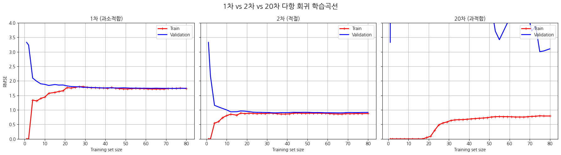

1차 함수에서는 훈련 검증의 RMSE둘다 높아 과소적합임

2차 함수에서는 훈련 검증의 RMSE가 둘다 낮음

3차 함수에서는 훈련 데이터는 RMSE가 낮지만, 검증데이터는 RMSE가 매우큼. 둘의 간격이 큼(과대적합)

 

4.5 규제가 있는 선형 모델

모델의 과대 적합을 줄이는 방법 중, 모델의 규제를 하는 방법입니다.

즉 가중치의 전체 크기를 줄입니다. 가중치가 크다는 것은 작은 x값의 변화에 예측값이 크게 변한다는 이야기이고, 지나치게 잘 맞추기 위해 복잡한 곡선을 그린다는 의미로 해석할 수 있습니다.

이는 훈련 데이터는 정확하지만, 새로운 데이터에는 부정확한 일반화 성능이 낮아집니다. 

규제(regurarization)은 가중치의 전체 크기를 억제해서 모델이 너무 복잡해지지 않도록 제어합니다.

 

가중치를 규제하는 방식에 따라, 대표적으로 아래 3개의 선형모델이 사용됩니다.

모델	규제방식	특징
릿지 회귀 (Ridge)	L2 규제: $\lambda \sum \theta_j^2$​	모든 가중치를 조금씩 줄임
라쏘 회귀 (Lasso)	L1 규제: ($\lambda \sum$	$\theta_j$
엘라스틱넷 (Elastic Net)	L1 + L2 혼합	Lasso와 Ridge의 장점 혼합

 

1) 릿지 회귀 (Ridge Regression)
$J(\theta) = \frac{1}{m} \sum_{i=1}^{m} \left( h_\theta(x^{(i)}) - y^{(i)} \right)^2 + \alpha \sum_{j=1}^{n} \theta_j^2$
L2 규제
가중치 제곱합에 패널티를 부여

2) 라쏘 회귀 (Lasso Regression)
$J(\theta) = \frac{1}{m} \sum_{i=1}^{m} \left( h_\theta(x^{(i)}) - y^{(i)} \right)^2 + \alpha \sum_{j=1}^{n} \left| \theta_j \right|$
L1 규제
가중치 절댓값의 합에 패널티
일부 가중치를 0으로 만들어 특성 선택 효과 있음

3) 엘라스틱넷 (Elastic Net)
$J(\theta) = \frac{1}{m} \sum_{i=1}^{m} \left( h_\theta(x^{(i)}) - y^{(i)} \right)^2 + \alpha \left( r \sum_{j=1}^{n} \left| \theta_j \right| + \frac{1 - r}{2} \sum_{j=1}^{n} \theta_j^2 \right)$
L1 + L2 혼합 규제

 

import numpy as np
import matplotlib.pyplot as plt
from sklearn.linear_model import Ridge, Lasso, ElasticNet
from sklearn.pipeline import make_pipeline
from sklearn.preprocessing import PolynomialFeatures, StandardScaler

# 데이터 생성
np.random.seed(42)
m = 20
X = 3 * np.random.rand(m, 1)
y = 1 + 0.5 * X + np.random.randn(m, 1) / 1.5
X_plot = np.linspace(0, 3, 100).reshape(-1, 1)

# 설정
alphas = [0, 0.01, 1]
poly_degree = 10
models = {
    "Ridge": Ridge,
    "Lasso": Lasso,
    "ElasticNet": ElasticNet
}

# 지수 표기 방지 설정
np.set_printoptions(suppress=True, precision=3)

# 가중치 출력 및 시각화 준비
print("가중치 비교 (다항 회귀 degree=10)")
print("=" * 50)
fig, axes = plt.subplots(1, 3, figsize=(18, 5), sharey=True)

for ax, (model_name, model_cls) in zip(axes, models.items()):
    print(f"\n {model_name}")
    for alpha in alphas:
        if model_name == "ElasticNet":
            model = make_pipeline(
                PolynomialFeatures(degree=poly_degree, include_bias=False),
                StandardScaler(),
                model_cls(alpha=alpha, l1_ratio=0.5, max_iter=10000)
            )
        else:
            model = make_pipeline(
                PolynomialFeatures(degree=poly_degree, include_bias=False),
                StandardScaler(),
                model_cls(alpha=alpha, max_iter=10000)
            )

        model.fit(X, y)
        final_model = model.named_steps[model.steps[-1][0]]
        coef = final_model.coef_.ravel()

        print(f"\u03B1 = {alpha:<4} → 가중치 개수: {len(coef)}")
        print(np.round(coef, 3))

        y_plot = model.predict(X_plot)
        ax.plot(X_plot, y_plot, label=f"\u03B1={alpha}")

    ax.scatter(X, y, c="k", s=20, label="data")
    ax.set_title(f"{model_name} (degree={poly_degree})")
    ax.set_xlabel("x")
    ax.grid(True)
    ax.legend()

axes[0].set_ylabel("y")
plt.suptitle("Regularization Effect on Polynomial Regression")
plt.tight_layout()
plt.show()

​

가중치 비교 (다항 회귀 degree=10)
==================================================

 Ridge
α = 0    → 가중치 개수: 10
[      6.208      31.46     -334.505   -1574.601   20066.351  -73236.371
  135003.079 -136919.936   72931.624  -15972.771]
α = 0.01 → 가중치 개수: 10
[ 1.225 -2.528  0.756  1.281  0.46  -0.402 -0.798 -0.633  0.03   1.077]
α = 1    → 가중치 개수: 10
[ 0.192 -0.052 -0.052 -0.028 -0.005  0.019  0.045  0.073  0.103  0.134]

 Lasso
α = 0    → 가중치 개수: 10
[  3.412 -12.833  13.317   2.253  -3.063  -3.563  -2.219  -0.458   1.169
   2.472]
α = 0.01 → 가중치 개수: 10
[ 0.132 -0.    -0.    -0.     0.     0.     0.     0.     0.     0.291]
α = 1    → 가중치 개수: 10
[0. 0. 0. 0. 0. 0. 0. 0. 0. 0.]

 ElasticNet
α = 0    → 가중치 개수: 10
[  3.412 -12.833  13.317   2.253  -3.063  -3.563  -2.219  -0.458   1.169
   2.472]
α = 0.01 → 가중치 개수: 10
[ 0.196 -0.077 -0.    -0.    -0.     0.     0.     0.     0.001  0.313]
α = 1    → 가중치 개수: 10
[0. 0. 0. 0. 0. 0. 0. 0. 0. 0.]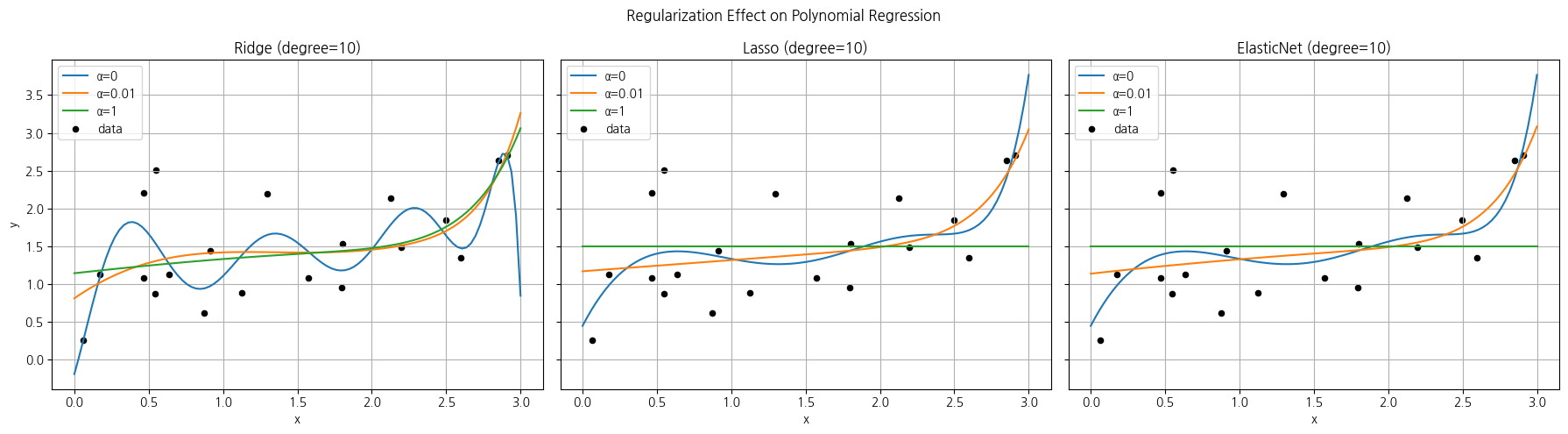

 

Ridge(L2규제) 

α 가 0일 때 고차항이 크고 진동이 심해 과적합입니다. 0.01, 1로 갈수록 곡선이 부드러워지고 안정화되어 일반화가 향상됩니다.

가중치는 전체적으로 작아집니다.

 

Lasso(L1 규제) 

α 가 0일 때 고차항이 크고 진동이 심해 과적합입니다. 0.01 시 변수 선택되어 가중치가 0인 항목들이 많아집니다. 1일때 모둔 가중치가 0으로 되었습니다.

 

4) 조기종료

훈련 도중에 검증 성능이 악화되기 시작하면 학습을 멈추는 방법

훈련 에포크 수 자체를 규제로 사용하는 것

에포크가 너무짧으면 과소적합, 너우 길면 과적합이 발생됩니다.

조기종료는 검증 손실이 최소가 되는 시점을 찾아 학습을 중단하는 방식입니다.

 

예제

from sklearn.linear_model import SGDRegressor

sgd = SGDRegressor(early_stopping=True, validation_fraction=0.1, n_iter_no_change=5)

 

 

4.6 로지스틱 회귀

로지스틱 회귀는 회귀가 아니라 분류에 사용됩니다.

입력 특성들의 선형조합을 계산 한 뒤, 결과값 시그모이드(sigmoid function)함수를 적용해서 0과 1사이의 확률로 변환합니다.

 

$σ(z)=\frac{1}{1+e^{−z}}$​

예측결과

\[
\hat{y} =
\begin{cases}
1 & \text{if } \hat{p} \geq 0.5 \\
0 & \text{otherwise}
\end{cases}
\]

 

로지스틱 회귀의 비용함수

\[
J(\theta) = -\frac{1}{m} \sum_{i=1}^m \left( y^{(i)} \log\left( \hat{p}^{(i)} \right) + \left(1 - y^{(i)}\right) \log\left( 1 - \hat{p}^{(i)} \right) \right)
\]

수식은 Binary Cross-Entropy Loss 또는 Log Loss로 불립니다.

 

정답 y는 0또는 1이고, 예측값은 0과 1사이에 확률로, 정답게 가까우면 작은값을, 틀린값이면 패털리가 급격히 커지게 됩니다.

 

경사하강을 적용하기 위해서는 시그모이드를 미분해야합니다.

$σ(z)=\frac{1}{1+e^{−z}}$

이를 미분하면 

\[
\frac{d}{dz} \sigma(z) = \sigma(z) \left( 1 - \sigma(z) \right)
\]

시그모이드 함수의 미분은 자기자신 X (1-자기자신)형태입니다.

 

다시한번 비용함수를 확인 시 아래와 같습니다.

\[
J(\theta) = -\frac{1}{m} \sum_{i=1}^{m} \left( y^{(i)} \log\left( \hat{p}^{(i)} \right) + (1 - y^{(i)}) \log\left( 1 - \hat{p}^{(i)} \right) \right)
\]

 

이를 미분하면

\[
\nabla_{\theta} J(\theta) = \frac{1}{m} \sum_{i=1}^{m} \left( \hat{p}^{(i)} - y^{(i)} \right) \mathbf{x}^{(i)}
\]

 

코드로 표시하면 아래와 같습니다.

import numpy as np

def sigmoid(z):
    return 1 / (1 + np.exp(-z))

def sigmoid_derivative(z):
    s = sigmoid(z)
    return s * (1 - s)

# 예시
z = np.array([0, 2, -2])
print("Sigmoid:", sigmoid(z))
print("Sigmoid 미분:", sigmoid_derivative(z))

Sigmoid: [0.5        0.88079708 0.11920292]
Sigmoid 미분: [0.25       0.10499359 0.10499359]

 

4.6.3 결정 경계(Decision Boundary)

결정 경계는 모델이 클래스를 구분하는 가상의 경계선입니다.

로지스틱에서는 p = 0.5를 경계로, 이보다 작으면 0 크면 1로 분류합니다.

2차원은 직선, 3차원은 평면, 고차원에서는 초평면(hyperplane)로 분류됩니다.

 

setosa와 versicolor로 결정경계 확인

import numpy as np
import matplotlib.pyplot as plt
from sklearn import datasets
from sklearn.linear_model import LogisticRegression

# 1. 데이터 불러오기
iris = datasets.load_iris()
X = iris["data"][:, (2, 3)]  # 꽃잎 길이, 꽃잎 너비만 사용
y = (iris["target"] == 0).astype(int)  # setosa이면 1, 아니면 0

# 2. 로지스틱 회귀 모델 훈련
model = LogisticRegression()
model.fit(X, y)

# 3. 결정 경계 그리기
x0, x1 = np.meshgrid(
    np.linspace(X[:, 0].min()-1, X[:, 0].max()+1, 500),
    np.linspace(X[:, 1].min()-1, X[:, 1].max()+1, 500),
)
X_new = np.c_[x0.ravel(), x1.ravel()]
y_proba = model.predict_proba(X_new)[:, 1].reshape(x0.shape)

plt.figure(figsize=(8, 4))
plt.contourf(x0, x1, y_proba, cmap="coolwarm", alpha=0.8)
plt.contour(x0, x1, y_proba, levels=[0.5], linewidths=2, colors="black")
plt.scatter(X[:, 0], X[:, 1], c=y, edgecolors="k")
plt.xlabel("Petal length")
plt.ylabel("Petal width")
plt.title("Logistic Regression Decision Boundary")
plt.colorbar()
plt.show()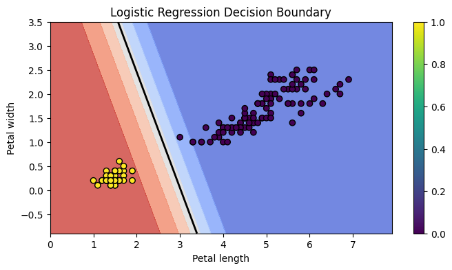

 

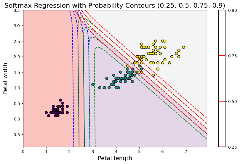
4.6.4 소프트맥스 회귀

2개 이상의 클래스를 분류하는 다항 로지스틱 회귀(Multinomial Logistic Regression)에서는 각 클래스마다 점수를 계산하고 소프트맥스 함수로 결과를 확률로 변환 합니다.

소프트 맥스 회귀는 여러 클래스를 다루는 로지스틱 회귀의 확장입니다.

 

1) 각 클래스 k의 logit score를 계산합니다.

\[
s_k(\mathbf{x}) = \theta_k^T \mathbf{x}
\]

2) 결과를 softmax함수로 확률로 변환합니다.

     소프트 맥스는 score들을 지수 변환 후 , 전체 합으로 나눕니다. 결과 0~1의 사이의 확률값으로 표시됩니다.

\[
\hat{p}_k = \frac{e^{s_k(\mathbf{x})}}{\sum_{j=1}^{K} e^{s_j(\mathbf{x})}}
\]

3) 결과값중 가장 확률이 큰것으로 예측합니다.

\[
\hat{y} = \arg\max_k \hat{p}_k
\]

4) 비용함수는 Cross Entropy를 사용합니다. 

\[
J(\theta) = -\frac{1}{m} \sum_{i=1}^{m} \sum_{k=1}^{K} y_k^{(i)} \log\left( \hat{p}_k^{(i)} \right)
\]

import numpy as np
import matplotlib.pyplot as plt
from sklearn import datasets
from sklearn.linear_model import LogisticRegression

# 1. 데이터 불러오기
iris = datasets.load_iris()
X = iris["data"][:, (2, 3)]  # 꽃잎 길이, 꽃잎 너비
y = iris["target"]

# 2. 소프트맥스 회귀 모델 훈련
softmax_reg = LogisticRegression(multi_class="multinomial", solver="lbfgs", C=10)
softmax_reg.fit(X, y)

# 3. 결정 경계와 소프트맥스 확률 계산
x0, x1 = np.meshgrid(
    np.linspace(X[:, 0].min() - 1, X[:, 0].max() + 1, 500),
    np.linspace(X[:, 1].min() - 1, X[:, 1].max() + 1, 500),
)
X_new = np.c_[x0.ravel(), x1.ravel()]
y_pred = softmax_reg.predict(X_new).reshape(x0.shape)
y_proba = softmax_reg.predict_proba(X_new)

# 클래스별 확률
proba_class0 = y_proba[:, 0].reshape(x0.shape)
proba_class1 = y_proba[:, 1].reshape(x0.shape)
proba_class2 = y_proba[:, 2].reshape(x0.shape)

# 4. 시각화
plt.figure(figsize=(10, 6))
plt.contourf(x0, x1, y_pred, cmap="Pastel1", alpha=0.8)  # 배경 결정영역
plt.scatter(X[:, 0], X[:, 1], c=y, edgecolor="k", s=40)  # 데이터 포인트

# 클래스별 확률 contour 추가
contour_levels = [0.25, 0.5, 0.75, 0.9]

plt.contour(x0, x1, proba_class0, levels=contour_levels, colors="blue", linestyles="dashed")
plt.contour(x0, x1, proba_class1, levels=contour_levels, colors="green", linestyles="dashed")
plt.contour(x0, x1, proba_class2, levels=contour_levels, colors="red", linestyles="dashed")

plt.xlabel("Petal length", fontsize=14)
plt.ylabel("Petal width", fontsize=14)
plt.title("Softmax Regression with Probability Contours (0.25, 0.5, 0.75, 0.9)", fontsize=16)
plt.colorbar()
plt.show()