
Transformer는 2017년 도입된 딥러닝 모델로, Attention 계층만으로 단어 간의 관계를 학습하여 처리하는 병렬처리가 가능하도록 설계된 모델입니다.
BERT, GPT등이 Transformer구조를 기반으로 만들어졌습니다.
논문 Attention Is All You Need 내용에 대한 스터디 정리
https://arxiv.org/abs/1706.03762
Attention Is All You Need
The dominant sequence transduction models are based on complex recurrent or convolutional neural networks in an encoder-decoder configuration. The best performing models also connect the encoder and decoder through an attention mechanism. We propose a new
arxiv.org
2017년 Attention is all you need논문의 내용을 기반으로 실제 코드로 구현합니다.
코드 작성 후 Toyset 시험 데이터를 생성 후 훈련 및 평가를 수행합니다.
작성 코드는 https://nlp.seas.harvard.edu/2018/04/03/attention.html 를 참조하여, 이해한 바를 바탕으로 새로 작성하였습니다. 따라서 일부 오류가 있을 수 있습니다.
Transform의 동작원리를 확인하려는 목적으로, 실제 사용하기 위해서는 많은 수정이 필요할 수 있습니다.

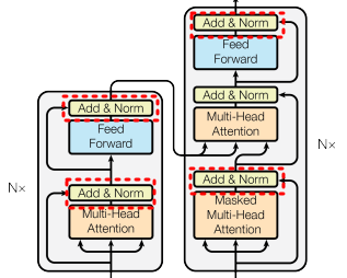
그림에서 Transformer는 다음의 단계를 수행합니다.
1. Input Embedding : 입력 단어를고정 크기의 벡터로 변환
2. Positional Encoding : 단어의 위치 정보를 임베딩에 추가
3. Self Attention & Multi Attention : 입력 간의 관계를 계산해 각 단어에 Attention score(중요도)계산
4. Add & Norm : 정규화
5. Feed-Forward Network : 각 단어 벡터를 독립적으로 학습
6. Output : 디코더를통해 결과 시퀀스를 생성
Attention이란?
먼저 Transform의 근간이 된 Attention에 대해 알아봅시다.
→ 문장 내의 단어들간의 중요도를 Query, Key, Value 의 3개의 벡터를 활용해 점수(Score)를 계산하는 방식입니다.
→ 일반적으로 생각하는 Query(검색어), 파이썬의 dictionary의 key와 value가 아니다 모두 동일한 크기(n)의 벡터입니다.
→ 3개의 벡터를 softmax( Q@K.T/ sqrt(d_k) ) @V 벡터 연산으로 아래 3개의 역할이 부여됩니다.
- Query: 현재 단어(토큰)가 다른 단어와 얼마나 관련 있는지 판단
- Key: 각 단어의 특징 벡터로, Query와의 유사도를 계산하는 기준.
- Value: 실제 정보를 담은 벡터로, Attention결과에 따라 가중합을 계산
Attention에 4가지 개념이 있습니다.
(1) Self-Attention : 모두 같은 데이터에서 Query, Key, Value를 생성해 단어간의 관계를 학습하는 Attention입니다.
(2) Sorce-Target Attention : Decoder의 Query와 Encoder의 Key, Value를 사용해 Source단어와 Target단어간 관계 학습.
(3) Scaled Dot-Producted Attention : Query와 Key의 내적을 계산 각 단어의 중요도를 측정, 이를 Value에 반영 출력 생성 .
(4) Multi-head Attention : 여러개의 독립적인 Attention을 병렬로 수행 후, 결과를 결합하여 학습 하는 개념입니다.
| 유형 | 특징 | 주요 활용 |
| Self-Attention | 같은 시퀀스 내에서 단어 간 관계 학습 | Transformer Encoder & Decoder |
| Source-Target Attention | 다른 시퀀스 간의 관계 학습 (예: 번역 모델에서 Source와 Target) |
Transformer Decoder |
| Scaled Dot-Product Attention |
Attention Score 계산 방식 | 모든 Attention 메커니즘의 핵심 |
| Multi-head Attention | 여러 Attention을 병렬적으로 계산하여 다양한 관계 학습 | Transformer 전체 (Encoder&Decoder) |
아래는 논문의 Scaled-Dot prroduct와 Multi-head attention의 블럭도 입니다.

(1) Self Attention
- 개념: 입력 시퀀스의 각 단어가 동일한 입력 시퀀스 내에서 다른 단어와의 관계를 평가하여 문맥을 학습합니다. 즉 문법 구조나 단어간의 관계성을 습득하는데 사용됩니다.
- 적용: 주로 Transformer에서 Encoder와 Decoder에서 사용됩니다.
- 핵심 단계:
- 입력 벡터를 Query, Key, Value로 변환 (선형 변환).
- Query와 Key의 내적 계산을 통해 각 단어 간의 연관성(Attention Score)을 도출.
- Attention Score를 Softmax로 정규화.
- 정규화된 Score를 Value에 가중합.
(2) Sorce-Target Attention
- 개념: 서로 다른 두 시퀀스 간의 상호작용을 학습합니다. (입력과 메모리)
- 예: 번역 모델에서 Source(입력 문장)와 Target(출력 문장)의 관계를 학습.
- 특징:
- Query는 Target/Decoder에서 생성(Input), Key와 Value는 Source(Enoder 출력)에서 생성.
- Self-Attention과 달리 입력과 출력 시퀀스가 다릅니다.
- 적용: Transformer에서 Decoder 단계에서 Source 문장을 고려해 Target 문장을 생성할 때 사용.
(3) Scaled Dot Product Attention
개념: Attention 메커니즘의 핵심 수학적 연산입니다.
장점: 단순하고 효율적인 Attention Score 계산 방식.

Mask는 문장을 처리할 때 다음 단어를 미리 예측하거나 보는 것을 막기 위한 역할입니다. 특정 상황에서 특정 Key의 영향을 배제하기 위해 Attention weight 를 0으로 만듭니다.
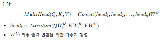
(4) Multi-Head Attention
- 개념: Attention을 병렬적으로 여러 개 계산하여 다양한 표현을 학습하는 방식.
- 각각의 Attention을 Head라고 합니다.
- 구조:
- 입력 벡터를 여러 개의 Query, Key, Value로 나눔.
- 각 쌍에 대해 독립적인 Scaled Dot-Product Attention 계산.
결과를 Concatenate하고 다시 선형 변환으로 결합합니다.
Multi-Head Attention을 사용하는 이유는 QW, KW, VW의 각각의 초기 가중치가 다른 경우 각각의 특성을 학습하여 이를 앙상블 개념으로, 성능을 높히는 기법입니다. 논문에서는 Mult-Head에 의한 성능 향상이 언급되어 있습니다.
Attention을 코드로 구현
Scaled Dot-Producted Attention
import torch
import torch.nn as nn
import torch.nn.functional as F

def scaled_dot_product_attention(Q, K, V, mask=None, dropout=None):
    """
    Scaled Dot-Product Attention 구현
    Args:
        Q (Tensor): Query, shape [batch_size, seq_len, d_k]
        K (Tensor): Key, shape [batch_size, seq_len, d_k]
        V (Tensor): Value, shape [batch_size, seq_len, d_v]
        mask (Tensor, optional): 마스크 텐서, shape [batch_size, seq_len, seq_len]

    Returns:
        output (Tensor): Attention 결과, shape [batch_size, seq_len, d_v]
        attention_weights (Tensor): Attention 가중치, shape [batch_size, seq_len, seq_len]
    """

    # Query와 Key의 행렬곱
    d_k = Q.size(-1)
    attention_scores = torch.matmul(Q, K.transpose(-2, -1))  # 마지막 2개 차원을 전치
    attention_scores = attention_scores / (d_k**0.5)  # Scaling 적용

    # 마스크 적용
    if mask is not None:
        attention_scores = attention_scores.masked_fill(mask == 0, float('-inf'))

    # Attention weights 계산 (Softmax)
    attention_weights = F.softmax(attention_scores, dim=-1) # [batch_size, seq_len, seq_len]
    if dropout is not None:
        attention_weights = dropout(attention_weights)

    # Attention weights와 Value의 가중합 계산
    output = torch.matmul(attention_weights, V) # [batch_size, seq_len, d_v]
    return output, attention_weights
Multi-Head Attention
class MultiHeadAttention(nn.Module):
    def __init__(self, d_model, n_head, dropout=0.1):
        """
        Multi-Head Attention 초기화
        Args:
            d_model (int): 전체 모델 차원
            n_head (int): Head의 개수
            dropout (float): 드롭아웃 비율
        """
        super().__init__()
        self.d_model = d_model
        self.n_head = n_head
        self.d_k = d_model // n_head  # 각 Head의 차원

        # Query, Key, Value에 대한 선형 변환 계층
        self.Q = nn.Linear(d_model, d_model, bias=False)
        self.K = nn.Linear(d_model, d_model, bias=False)
        self.V = nn.Linear(d_model, d_model, bias=False)
        self.Output = nn.Linear(d_model, d_model, bias=False)
        self.dropout = nn.Dropout(p=dropout)

        # Attention 가중치를 저장할 변수
        self.attention = None

    def forward(self, Q, K, V, mask=None):
        """
        Multi-Head Attention Forward 연산
        Args:
            Q (Tensor): Query, shape [batch_size, seq_len, d_model]
            K (Tensor): Key, shape [batch_size, seq_len, d_model]
            V (Tensor): Value, shape [batch_size, seq_len, d_model]
            mask (Tensor, optional): 마스크 텐서, shape [batch_size, seq_len, seq_len]

        Returns:
            output (Tensor): Multi-Head Attention 결과, shape [batch_size, seq_len, d_model]
            attention_weights (Tensor): Attention 가중치, shape [batch_size, n_head, seq_len, seq_len]
        """
        batch_size = Q.size(0)

        # Query, Key, Value를 Head 개수(n_head)로 나누고 차원을 변환
        Q = self.Q(Q).view(batch_size, -1, self.n_head, self.d_k).transpose(1, 2)
        K = self.K(K).view(batch_size, -1, self.n_head, self.d_k).transpose(1, 2)
        V = self.V(V).view(batch_size, -1, self.n_head, self.d_k).transpose(1, 2)

        # 마스크 차원을 Head에 맞게 확장
        if mask is not None:
            mask = mask.unsqueeze(1)  # [batch_size, 1, seq_len, seq_len]

        # Scaled Dot-Product Attention 적용
        x, self.attention = scaled_dot_product_attention(Q, K, V, mask=mask, dropout=self.dropout)

        # Head를 결합(concatenate)하고 최종 선형 변환 적용
        x = x.transpose(1, 2).contiguous().view(batch_size, -1, self.d_model)
        output = self.Output(x)

        return output, self.attention
Transformer에서는 Scaled Dot Attention을 병렬로 n_head 회 각각 수행한 뒤, 그결과를 합쳐 사용합니다.
n_head는 병렬로 처리하는 헤더의 개수입니다. d_k * h를 d_model로 사용합니다.
x = x.transpose(1, 2).contiguous().view(batch_size, -1, self.d_model)
- transpose: Head 차원을 시퀀스 길이 차원 뒤로 이동합니다.
- contiguous: 메모리 배치를 재정렬하여 연속된 상태로 만듦니다.
- view: 여러 Head의 출력를 모양을 다시 batch_size,seq_len,d_model 형식으로 재배치합니다.
- X = torch.cat([head1, head2], dim=-1) 식으로 concat할 수 있지만, Multi-Head Attention에서는 모든 Head가 하나의 텐서로 결합되어 있기 때문에, torch.cat 대신 view를 사용해 효율적으로 차원을 재구성합니다
Embedding
가장 중요한 Attention의 코드를 작성해보았으므로, Transformer의 나머지 각 부분을 작성해봅니다.
I like apple등의 문장이 들어오면, Embedding과정을 통해 Vector화 됩니다.
과정은 자연어 처리의 Word2Vector과 유사한, 항목들간의 유사도를 밀집 Vector형식으로 변경합니다.
Embedding Layer의 Input 은 정수형태로 입력되는데 Embedding Layer 이전에 별도의 라이브러리나, 함수로 전처리 후 정수형태로 입력됩니다.
from transformers import AutoTokenizer
tokenizer = AutoTokenizer.from_pretrained("bert-base-uncased")

# 입력 문장
text = "I like apples"
# 토큰화 및 인덱싱
encoded = tokenizer(text, return_tensors="pt")  # PyTorch 텐서 반환
어떻게 입력되는지 이해되도록 간단한 함수를 작성해보면 아래와 같습니다.
vocab = {"I": 0, "like": 1, "apples": 2, "bananas": 3, "and": 4}  # 사전 정의

def tokenize_and_index(text, vocab):
    tokens = text.split()  # 간단한 토큰화
    return [vocab[token] for token in tokens if token in vocab]

# 텍스트 예제
text = "I like apples"
token_ids = tokenize_and_index(text, vocab)
print("Token IDs:", token_ids)  # [0, 1, 2]

# 임베딩 레이어 정의
vocab_size = len(vocab)
d_model = 8  # 임베딩 벡터 차원
embedding_layer = nn.Embedding(num_embeddings=vocab_size, embedding_dim=d_model)

# 텐서로 변환
input_tensor = torch.tensor(token_ids).unsqueeze(0)  # [batch_size, seq_len]
print("Input Tensor Shape:", input_tensor.shape)  # [1, 3]

# 임베딩 계산
output = embedding_layer(input_tensor)
print("Embedding Output Shape:", output.shape)  # [1, 3, d_model]
Embedding은 단어를 벡터화하는 Token Enbedding함수 nn.Embedding()를 사용하여 구현할 수 있습니다.
nn.Embedding은 단어를 벡터화 하는 자연어 처리작업에 주로 사용됩니다.
import torch
import torch.nn as nn
import math

class Embeddings(nn.Module):
    def __init__(self, vocab_size, d_model):
        """
        임베딩 계층 초기화
        Args:
            d_model (int): 모델 차원
            vocab_size (int): 어휘 크기, 단어들의 토큰 개수
        """
        super().__init__()
        self.embedding = nn.Embedding(num_embeddings=vocab_size, embedding_dim=d_model)
        self.d_model = d_model

    def forward(self, x):
        """
        임베딩 벡터와 스케일링 반환
        Args:
            x (Tensor): 입력 시퀀스, shape [batch_size, seq_len]

        Returns:
            Tensor: 스케일된 임베딩 벡터, shape [batch_size, seq_len, d_model]
        """
        # 임베딩 계산 및 스케일링 적용
        return self.embedding(x) * math.sqrt(self.d_model)
self.embedding(x) * math.sqrt(self.d_model)
- 입력 데이터를 d_model차원의 임베딩 벡터로 변환합니다. d_model 차원이라, 벡터의 크기가 1/(d_model**0.5)로 설정되어 초기 임베딩 크기가 너무 작아집니다. 이를 보정하기 위해 math.sqrt(self.d_model) 를 곱해 입력의 크기를 조정합니다.
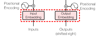
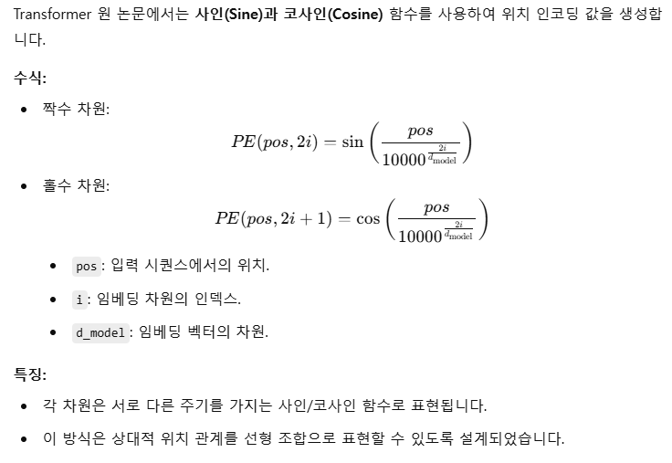
Positional Encoding
모델이 입력 시퀀스 내에서 단어의 위치 정보를 학습하도록 돕는 방법
Transformer는 Attention 메커니즘을 사용하여 입력 시퀀스의 모든 토큰을 병렬로 처리합니다. 이 과정에서 토큰 간 상대적 또는 절대적 위치 정보를 반영하기 위해 Positional Encoding을 추가합니다.
- Attention 메커니즘은 단어 간의 관계를 학습하지만, 단어의 순서 정보는 인지하지 못합니다.
- 이를 보완하기 위해 Positional Encoding이 입력 임베딩에 더해져 모델이 순서와 관련된 정보를 학습할 수 있습니다.
1. Input
["I", "love", "transformers"]

Input Embedding : nn.Embedding
["I" → [0.1, 0.5], "love" → [0.3, 0.7], "transformers" → [0.6, 0.8]]

2. Positional Encoding 값 생성
pos=0 → [sin(0), cos(0)]
pos=1 → [sin(0.0001), cos(0.0001)]
pos=2 → [sin(0.0002), cos(0.0002)]

3. Input + Positional Encoding : 입력 임베딩과 Positional Encoding을 더함
Final Input = Embedding + Positional Encoding
코드로 구현해보기
import torch
import torch.nn as nn

class PositionalEncoding(nn.Module):
    def __init__(self, d_model, max_len=5000):
        """
        Positional Encoding 초기화
        Args:
            d_model (int): 모델 차원
            max_len (int): 최대 시퀀스 길이
        """
        super().__init__()

        # Positional Encoding 초기화
        self.encoding = torch.zeros(max_len, d_model)

        # 위치 인덱스 생성
        position = torch.arange(0, max_len, dtype=torch.float).unsqueeze(1)

        # 주기적 함수의 분모 계산
        div_term = torch.exp(torch.arange(0, d_model, 2).float() * -(torch.log(torch.tensor(10000.0)) / d_model))

        # 짝수 인덱스: sin, 홀수 인덱스: cos
        self.encoding[:, 0::2] = torch.sin(position * div_term)
        self.encoding[:, 1::2] = torch.cos(position * div_term)
        self.encoding = self.encoding.unsqueeze(0)  # 배치 차원 추가

    def forward(self, x):
        """
        Positional Encoding을 입력에 추가
        Args:
            x (Tensor): 입력 텐서, shape [batch_size, seq_len, d_model]
        Returns:
            Tensor: Positional Encoding이 추가된 텐서
        """
        # 디바이스 일치화
        self.encoding = self.encoding.to(x.device)

        # Positional Encoding 추가
        x = x + self.encoding[:, :x.size(1), :]
        return x
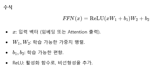
Feed Forward Neural Network(FFN)

2개의 전결합층과 ReLU로 구성된 층으로 각각의 단어와 위치별로 순전파로 학습합니다.
Attention 은 단어간의관계를 학습하지만, FFN은 입력된 각 단어 벡터를 독립적으로 변환하여, 단어 자체의 특징을 학습합니다. 즉 단어와의 영향을 배제하여, 각각의 단어의 관계를 고려하지 않습니다.
FFN의 가중치와 편향은(W1,W2, B1, B2)는 모든 네트워크에서 동일하게 사용됩니다. 이는 모델이 모든 위치에서 동일한 변환 규칙을 적용하도록 설계되었기 때문입니다.
FFN의 구현
import torch
import torch.nn as nn

class PositionwiseFeedForward(nn.Module):
    """
    Position-wise Feed Forward Network
    Args:
        d_model (int): 모델 차원
        d_ff (int): Feed Forward 레이어 내부 차원
        dropout (float): 드롭아웃 비율
    """
    def __init__(self, d_model, d_ff, dropout=0.1):
        super().__init__()
        self.W1 = nn.Linear(d_model, d_ff)  # 첫 번째 선형 변환
        self.W2 = nn.Linear(d_ff, d_model)  # 두 번째 선형 변환
        self.dropout = nn.Dropout(dropout)  # 드롭아웃 레이어
        self.relu = nn.ReLU()  # 활성화 함수

    def forward(self, X):
        """
        Args:
            X (Tensor): 입력 텐서, shape [batch_size, seq_len, d_model]
        Returns:
            Tensor: 출력 텐서, shape [batch_size, seq_len, d_model]
        """
        # 첫 번째 선형 변환과 활성화 함수
        X = self.W1(X)
        X = self.relu(X)

        # 드롭아웃 적용
        X = self.dropout(X)

        # 두 번째 선형 변환
        X = self.W2(X)
        return X
Layer Norm
Transformer에서 Layer Norm은 Add & Norm으로 사용되며, Add(잔차 연결, 이전 레이어의 출력값을 더함)과 Layer Normalization으로 수행됩니다.
레이어의 출력값의 분포를 정류화하여, 기울기 소실이나, 폭팔, 수렴속도 향상, 일반화 성능 향상의 이점을 제공합니다.
(1) Add (잔자연결)
Residual Output = Input + Layer Output
(2) Layer Normalization :

Transformat에서는 Batch Normalization대신 Layer Lormalization이 사용됩니다. 레이어 출력의 각 차원이 정규화 대상이 됩니다.
Layer Normalization, Jimmy Lei Ba, et al(2016 논문 참고)
PyTorch의 nn.LayerNorm 으로 Layer Normalization을 구현 할 수 있습니다.
# Add & Norm

import torch
import torch.nn as nn

class AddAndNorm(nn.Module):
    """
    Residual connection + Layer Normalization + Dropout
    """
    def __init__(self, d_model, dropout=0.1):
        """
        Args:
            d_model (int): 모델 차원
            dropout (float): Dropout 비율
        """
        super(AddAndNorm, self).__init__()
        self.norm = nn.LayerNorm(d_model)  # Layer Normalization
        self.dropout = nn.Dropout(dropout)  # Dropout

    def forward(self, x, sublayer=None):
        """
        Args:
            x (Tensor): Residual 입력 텐서, shape [batch_size, seq_len, d_model]
            sublayer (Callable, optional): 적용할 서브 레이어 (없을 경우 None)
        Returns:
            Tensor: Residual Connection + Dropout + Normalization 결과
        """
        if sublayer is None:
            # Sublayer가 없으면 Normalization만 적용
            return self.norm(x)

        # Sublayer를 적용하기 전에 입력 x를 정규화
        sublayer_output = self.norm(sublayer)

        # Dropout과 Residual Connection 적용
        return x + self.dropout(sublayer_output)
Transformer의 각 요소에 대해 구현해보았습니다.
다음 글에 각 요소를 합쳐서 Encoder, Decoder, Transformer를 작성해 보겠습니다.
'딥러닝' 카테고리의 다른 글
| 자동미분(automatic differentiation) (0) | 2025.07.19 |
|---|---|
| Transformer Section2 (1) | 2025.01.02 |
| 파이토치(Pytorch) 개요 (2) | 2024.11.20 |
| MLP (3) | 2023.10.04 |
| 인공신경망(ANN) (1) | 2023.08.10 |